第5回 MATLAB seminar 2021年07月06日
最終更新:2020/07/08
Introduction to Principal Component Analysis (PCA). Here, MATLAB code and the notes used in the seminar are shared.
In this article only basic fundamental examples are given. If you want to know more on it, please access the matlab website.
NOTE
You can download the notes used in the seminar from this link.
Example
Dataset
We use "load fisheriris" dataset.
load fisheriris.mat % load dataset
Check meas and species are loaded into your Workspace.
Type meas and species.
measis 4-dimension data for 150 iris (name of a flower) data.speciesis 1-dimension data for 150 iris (name of a flower) data. These are names of iris species.
meas % type it

% MATLAB OUTPUT
meas =

5.1000    3.5000    1.4000    0.2000
4.9000    3.0000    1.4000    0.2000
4.7000    3.2000    1.3000    0.2000
4.6000    3.1000    1.5000    0.2000
:

species % type it

% MATLAB OUTPUT
species =

150×1 cell array

{'setosa'    }
{'setosa'    }
{'setosa'    }
:
Normalize the data
Normalize the data for PCA.
d = normalize(meas) % type it

% OUTPUT (normalized data)
d =

 -0.8977    1.0156   -1.3358   -1.3111
 -1.1392   -0.1315   -1.3358   -1.3111
 -1.3807    0.3273   -1.3924   -1.3111
 -1.5015    0.0979   -1.2791   -1.3111
 -1.0184    1.2450   -1.3358   -1.3111
 -0.5354    1.9333   -1.1658   -1.0487
:
Carry out PCA
Extremely easy.
[COEFF, SCORE, LATENT] = pca(d);
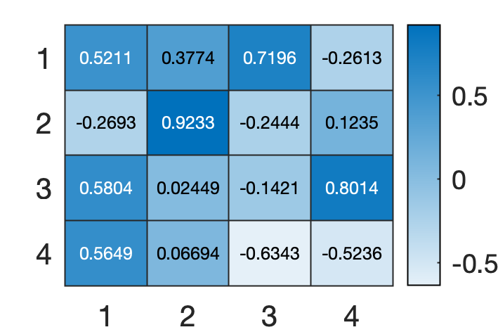
COEFF is a matrix to convert the data.
You can visualize the data for example,
heatmap(COEFF)
LATENT is a principal component variances.
You can compute contribution ratio for example,
cr = 100*LATENT / sum(LATENT);
disp(['Contribution ratio of the PC1 is ' num2str(cr(1)) ' %'])
disp(['Contribution ratio of the PC2 is ' num2str(cr(2)) ' %'])
disp(['Contribution ratio of the PC3 is ' num2str(cr(3)) ' %'])
disp(['Contribution ratio of the PC4 is ' num2str(cr(4)) ' %'])

% OUTPUT
Contribution ratio of the PC1 is 72.9624 %
Contribution ratio of the PC2 is 22.8508 %
Contribution ratio of the PC3 is 3.6689 %
Contribution ratio of the PC4 is 0.51787 %
SCORE is the data on the new axes.
You can compute contribution ratio for exmaple.
Please verify that the SCORE is also 150*4 Matrix.
SCORE

% OUTPUT
SCORE =

 -2.2571    0.4784    0.1273   -0.0241
 -2.0740   -0.6719    0.2338   -0.1027
 -2.3563   -0.3408   -0.0441   -0.0283
 -2.2917   -0.5954   -0.0910    0.0657
 -2.3819    0.6447   -0.0157    0.0358
 :
Visualization
If you want to visualize PC1 and PC2,
gscatter(SCORE(:, 1), SCORE(:, 2), species)
xlabel('PC1')
ylabel('PC2')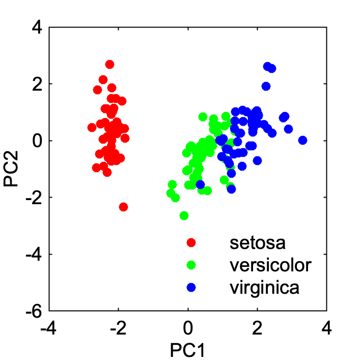
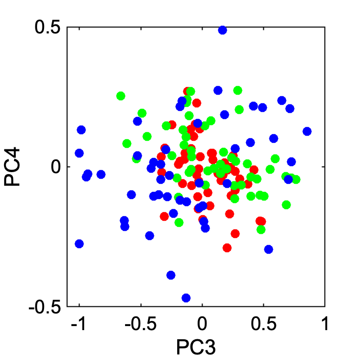
If you want to visualize PC3 and PC4,
gscatter(SCORE(:, 3), SCORE(:, 4), species)
xlabel('PC3')
ylabel('PC4')