『ゼロからできるMCMC』 Chapter7 Ising modelをJuliaで

最終更新：2020/12/7

『ゼロからできるMCMC』 Chapter7 Ising model(イジングモデル)のコードを, 練習を兼ねてJuliaで書いてみました. 私は, イジングモデルに関しては全く素人なので結果の解釈等については大きな錯誤があるかもしれません. また，詳細なことを書くと著作権的にだめな気もするので, 解説などはありません.

Version 1.6.2

Metropolis法によるサンプリング

Julia code

$N \times N$ 格子で温度は $T$, 結合定数は $J$, 外部磁場は $h$ としている. 初期状態はランダムに+1, -1を各格子に与えた. 格子点 $i_x$, $i_y$をランダムに選び, 確率 $\min{(1, \exp{(-\Delta E/T)})}$ でその格子 ( $s_{i_{x}, i_{y}}$ ) のスピンを反転させる. $\Delta E$ は,

\begin{align} \large \Delta E = 2 s_{i_{x}, i_{y}} \left( J \sum_{\pm 1} (s_{i_{x} \pm 1, i_{y}} + s_{i_{x}, i_{y} \pm 1}) + h \right) \tag{7.50} \end{align}

と計算した. 計算回数はNiterステップに一回のサンプリングとした. そして, Nprint回サンプルした.

境界条件は周期境界条件とした. 端っこに対応するために, nm, npという変数をつくっている. これは例えば $N = 5$ の場合だと,

nm = [5, 1, 2, 3, 4]
np = [2, 3, 4, 5, 1]

という配列である.

Julia

using Plots
using Random:seed!

## パラメータ
struct Params
    N::Int64
    Niter::Int64
    J::Float64
    h::Float64
    T::Float64
    Nprint::Int64
end

## 初期配位
function initializeState(N)
    # s = ones(N, N);
    s = randn(N, N); 
    @. s[s>0] = 1
    @. s[s<0] = -1
    return s
end

## ΔEの計算
function calcdE(s, J, h, ix, iy, np, nm)
    dE = 2*s[ix, iy] * (J*(s[np[ix], iy] + s[nm[ix], iy] + s[ix, np[iy]] + s[ix, nm[iy]])+h);
    return dE
end

## Metropolis法で更新
function isingMetropolis(p::Params)

    naccept = 0;
    s = zeros(p.N, p.N, p.Nprint);
    s[:, :, 1] = initializeState(p.N);
    np = [Vector(2:p.N); 1]
    nm = [p.N; Vector(1:p.N-1)];

    for I = 2:p.Nprint
        ss = s[:, :, I-1];
        for K = 1:p.Niter

            # select a random cell
            ix = rand(1:p.N);
            iy = rand(1:p.N);

            # calculate action
            dE = calcdE(ss, p.J, p.h, ix, iy, np, nm);

            # Metropolis test
            if exp(-dE/p.T) > rand()
                ss[ix, iy] = -ss[ix, iy];
                naccept += 1;
            end
        end
        s[:, :, I] = ss;
    end
    r = 100*naccept/(p.Nprint*p.Niter);
    display("acceptance rate is $(r) %")
    return s
end


## ここからメイン
p = Params(100, #N
           100^2*10, # Niter
           1.0, # J
           0.0, # h
           2/log(1+sqrt(2)), #T (crit: 2/log(1+sqrt(2)))
           100) # Nprint;
           
@time S = isingMetropolis(p::Params);

# gifとして保存
anim = Animation()
for I = 2:p.Nprint
    fig = heatmap(S[:, :, I], 
                  aspect_ratio=:equal, 
                  showaxis=:false,
                  grid=:false,
                  ticks = nothing,
                  size = (200, 200),
                  colorbar=:none)
    frame(anim, fig)
end
gif(anim, "ising3.gif", fps=10)

コード内に示したような設定で計算した. 0.454313 seconds (2.93 k allocations: 15.539 MiB)とのこと. 温度は相転移温度に設定した.

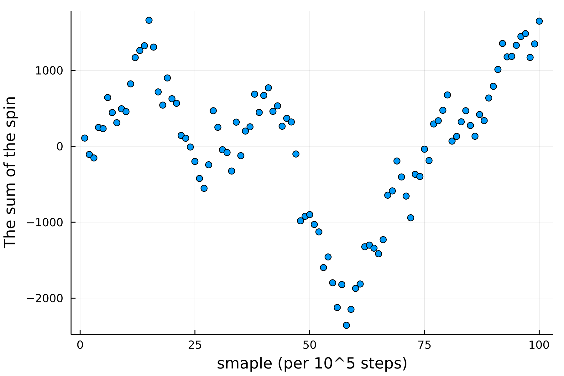
教科書には臨界減速の話が載っているので, このケースについても自己相関をみてみた. 荒いサンプリングで申し訳ないが, 相転移温度に設定したことによって強い自己相関が現れているのがわかる.

Juliaコード

Julia

spinSum = [sum(S[:, :, I]) for I in 1:p.Nprint]
plt =scatter(1:p.Nprint, spinSum)
xlabel!("smaple (per 10^5 steps)")
ylabel!("The sum of the spin")
plt[1][:legend] = :none
plt[:dpi] = 300;
png(plt, "ising4")

外部磁場の変化

結合定数 $J = 1$, 温度 $T=1$ に固定し, 外部磁場 $h$ を変化させてみる. 格子サイズは64, 40960ステップに一回のサンプリングとする. これは, 教科書図7.9の再現である.

初期状態はすべてのスピンが上向き ( ＋1 ) とする. そして, 初期の外部磁場は $h = -0.4$ で 100サンプルに一回磁場を 0.1下げ, 400回のサンプリングを行なう. なお, 外部磁場が負のときの基底状態はすべてのスピンが下向きである.

コードは, 磁場を下げるたびに ( 100回サンプルするたびに ) そのタイムステップまでの100回分のスピンの合計を計算している. また, そのあと前の100回の最後の状態を次の初期状態としないといけないので, 新たに上の節とは異なる函数をつくった. 絶対もっと効率的な方法があると思うが, Juliaは速いので気にならなかった.

Julia

function initializeState(S)
    s = S[:, :, end]
    return s
end

# 前の基底状態を引き継げるようにした函数
function isingMetropolisContinue(p::Params,  S)

    naccept = 0;
    s = zeros(p.N, p.N, p.Nprint);
    s[:, :, 1] = initializeState(S);
    np = [Vector(2:p.N); 1]
    nm = [p.N; Vector(1:p.N-1)];

    for I = 2:p.Nprint
        ss = s[:, :, I-1];
        for K = 1:p.Niter

            # select a random cell
            ix = rand(1:p.N);
            iy = rand(1:p.N);

            # calculate action
            dE = calcdE(ss, p.J, p.h, ix, iy, np, nm);

            # Metropolis test
            if exp(-dE/p.T) > rand()
                ss[ix, iy] = -ss[ix, iy];
                naccept += 1;
            end
        end
        s[:, :, I] = ss;
    end
    r = 100*naccept/(p.Nprint*p.Niter);
    display("acceptance rate is $(r) %")
    return s
end

# ここからがメイン
sumSpin = zeros(1, 400)
hs = [-0.4 -0.5 -0.6 -0.7];
S  = ones(64, 64, 1);
for H = 1:4
    p = Params(64, 64^2*10, 1.0, hs[H], 1.0, 100) 
    @time S = isingMetropolisContinue(p::Params,  S);
    sumSpin[1+100*(H-1):100*H]= [sum(S[:, :, I]) for I = 1:100]
end

#plot 
sumSpin = sumSpin’;
fig = scatter(1:100,    sumSpin[1:100],   markershape=:x, label="h=-0.4")
      scatter!(101:200, sumSpin[101:200], markershape=:x, label="h=-0.5")
      scatter!(201:300, sumSpin[201:300], markershape=:x, label="h=-0.6")
      scatter!(301:400, sumSpin[301:400], markershape=:x, label="h=-0.7")
xlabel!("iteration")
ylabel!("The sum of the spins")
png("ising1.img")

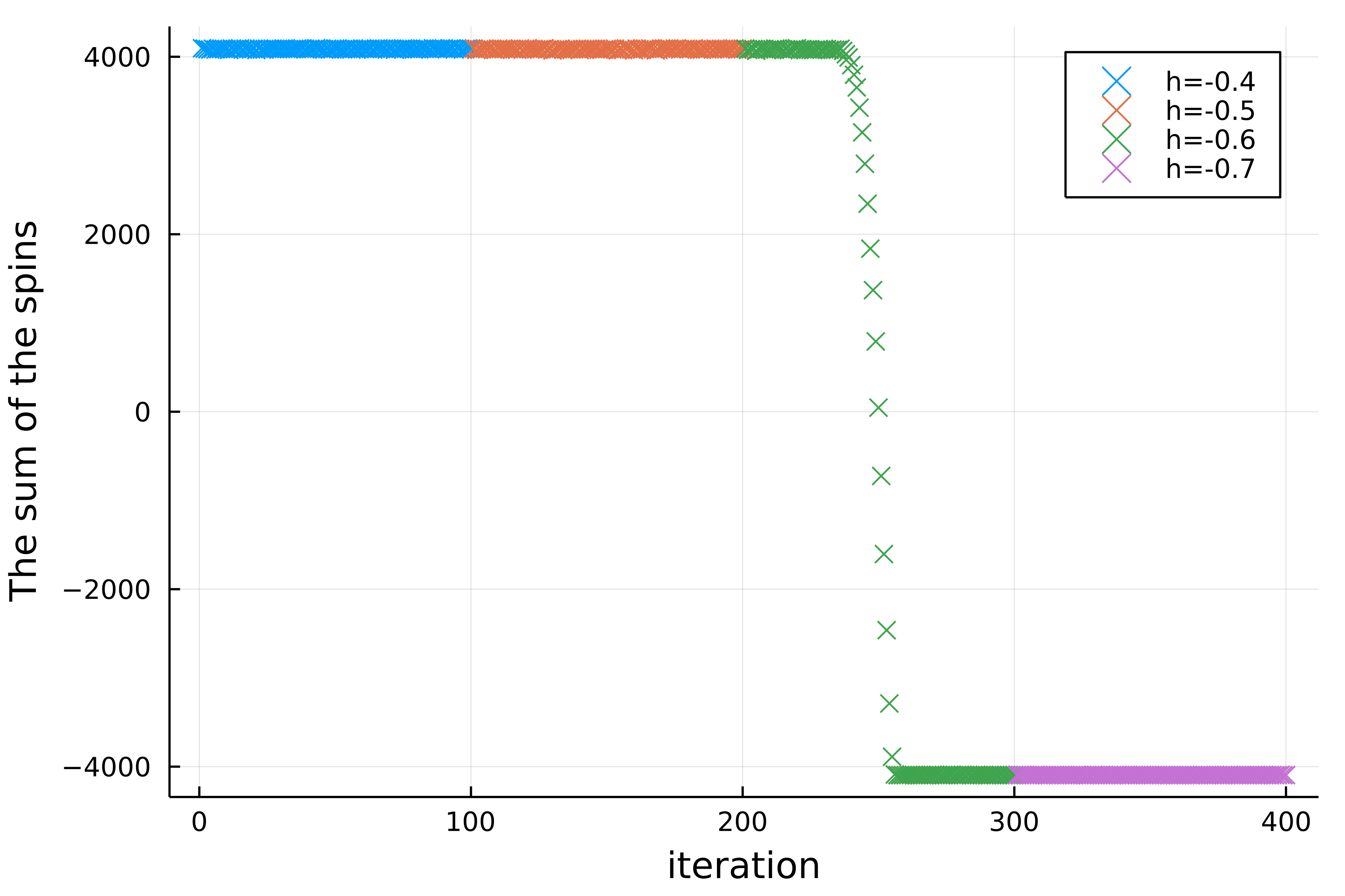
$h=-0.4$ ではなかなかスピンがすべて1の状態から抜け出せていない. $h=-0.6$ くらいまで下げてやっと基底状態 ( スピンがすべて−1, 即ちスピンの和は−4096 ) へ遷移し始める.

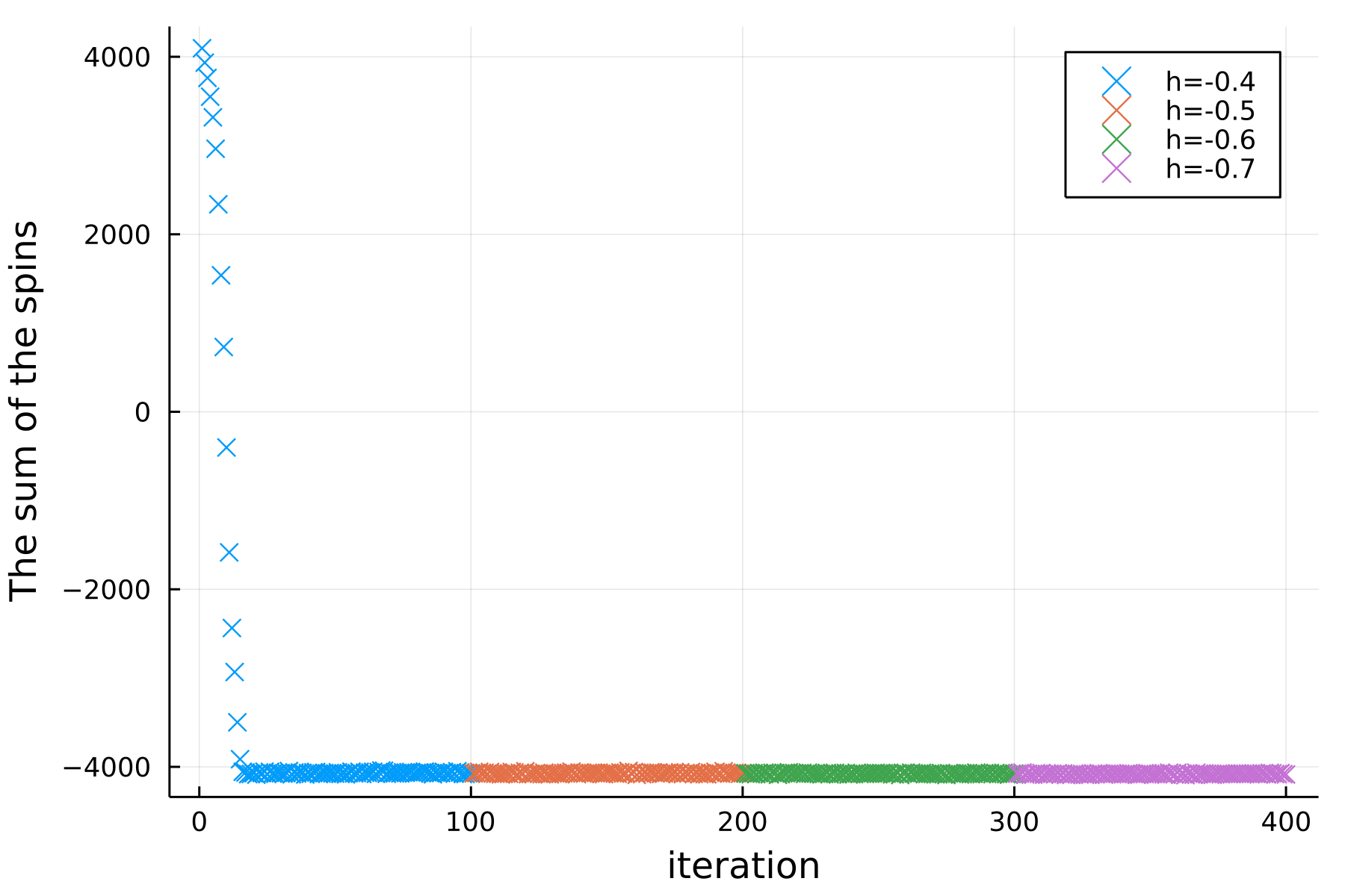
上の例は $T=1.0$ でのシミュレーションであった. $T=1.5$ と少し温度を上げてやると以下のように速やかに基底状態へ遷移する ( この辺の解釈については統計力学を勉強したことがないので自信がない ) .

Wolffのアルゴリズム

解説は教科書を見ていただきたい.

Julia

using Plots

## parameters
struct Params
    N::Int64
    nIter::Int64
    J::Float64
    T::Float64
    nPrint::Int64
end

function initializeState(N)
    s = randn(N, N); 
    @. s[s>0] = 1
    @. s[s<0] = -1
    return s
end

function isingWolff(p::Params)
    
    S = zeros(p.N, p.N, p.nPrint)      # preallocation
    S[:, :, 1] = initializeState(p.N)  # 初期状態を格納
    np = [Vector(2:p.N); 1]            # 1:1:Nに+１した値
    nm = [p.N; Vector(1:p.N-1)]        # 1:1:Nに-１した値
    prob  = 1 - exp(-2 * p.J / p.T)    # クラスタに追加する確率
    
    s = S[:, :, 1]                     # 初期状態から開始
    for J = 2:p.nPrint                 # p.nPrint回サンプリング
        for I = 1:p.nIter              # サンプリング毎にp.nIterステップ ( クラスタの反転 ) 行なう
            # クラスタを反転させる函数
            s = clusterFlip(prob, nm, np, p.N, s)
        end
        S[:, :, J] = s
        display(J)
    end
    return S
end


# クラスタを反転させる函数
function clusterFlip(prob, nm, np, N, s)
    inOrOut = falses(N, N)            # クラスタに各点が属するかの情報. 0 is out, 1 is out of the cluster ( 教科書と逆！ ) 
    ix = rand(1:p.N)                  # choose a random point
    iy = rand(1:p.N)
    inOrOut =  falses(N, N)           
    inOrOut[ix, iy] = true            # add the point to the cluster
    spinCluster = s[ix, iy]           # this cluster' spin (+1 or -1)
    iCluster = [ix iy]                # １つ目の点をクラスタに追加
    
    k = 1
    while k-1 < size(iCluster, 1)　   # ここからは教科書のコードとあまりかわらない
        ix, iy = iCluster[k, :]       # クラスタに属する点を選択
        ixp1 = np[ix]
        ixm1 = nm[ix] 
        iyp1 = np[iy] 
        iym1 = nm[iy]
        
        # 右隣
        # 次のif文は, 隣とスピンが同じでかつ, すでにクラスタに入っていない場合, ということ
        if s[ixp1, iy] == spinCluster && ~inOrOut[ixp1, iy]
            if rand() < prob
                iCluster = [iCluster; [ixp1 iy]]
                inOrOut[ixp1, iy] = true;
            end
        end
        
        # 上隣
        if s[ixm1, iy] == spinCluster && ~inOrOut[ixm1, iy]
            if rand() < prob
                iCluster = [iCluster; [ixm1 iy]]
                inOrOut[ixm1, iy] = true;
            end
        end
        
        # 左隣
        if s[ix, iyp1] == spinCluster && ~inOrOut[ix, iyp1]
            if rand() < prob
                iCluster = [iCluster; [ix iyp1]]
                inOrOut[ix, iyp1] = true;
            end
        end
        
        # 下隣
        if s[ix, iym1] == spinCluster && ~inOrOut[ix, iym1]
            if rand() < prob
                iCluster = [iCluster; [ix iym1]]
                inOrOut[ix, iym1] = true;
            end
        end
        k += 1
    end
        
    @. s[inOrOut] = -1*s[inOrOut] # クラスタに属する点をいっきに反転
    return s
end


## メイン
p = Params(200, #N
           10, # Niter
           1.0, # J
           2.30, #2/log(1+sqrt(2)), #T (crit: 2/log(1+sqrt(2)))
           350) # Nprint;
           
@time S = isingWolff(p)

# 動画で保存
anim = Animation()
for I = 2:p.nPrint
    fig = heatmap(S[:, :, I], 
                  aspect_ratio=:equal, 
                  showaxis=:false,
                  grid=:false,
                  ticks = nothing,
                  size = (200, 200),
                  colorbar=:none,
                  title="t = $(I)")
                  # c = :cividis) # お好きな色に
    frame(anim, fig)
end
gif(anim, "test.gif", fps=20)

上のコード内に示した条件での結果. どんどんクラスタが大きくなり, 最後は基底状態をいったりきたりする結果となった. 最後の方になると, 一つのクラスタが大きくなるからか, 計算時間が非常に長くなる. これは, コードが悪いのかそうなって当然なのかどうだろう. tが1進むごとに, 10ステップ進んでいることに注意.

この記事のTOP BACK TOP