『ゼロからできるMCMC』 Chapter 4をJuliaで
最終更新:2020/11/9
『ゼロからできるMCMC』 Chapter 4のコードを, 練習を兼ねてJuliaで書いてみました. 詳細なことを書くと著作権的にだめな気もするので, 解説などはありません.
Julia Version 1.5.0
Metropolis法を用いた\( S(x) = x^2/2 \)からのサンプル ( p.52 )
モンテカルロ法で円周率を求める.
Julia
using Random: seed!

function main(niter)

    seed!(12345)
    step_size = 0.5

    # initial values
    x = 0.0
    naccept = 0
    xs = zeros(Float64, niter)

    # main
    for i = 1:niter
        backup_x    = x
        action_init = 0.5*x*x
        x += (rand()-0.5)*step_size*2.0

        action_fin = 0.5*x*x

        # Metropolis test
        metropolis = rand()
        exp(action_init - action_fin) > metropolis ? naccept+= 1 : x=backup_x
        xs[i] = x
    end
    return xs
    naccept/niter
end
xsにサンプルを格納しました.
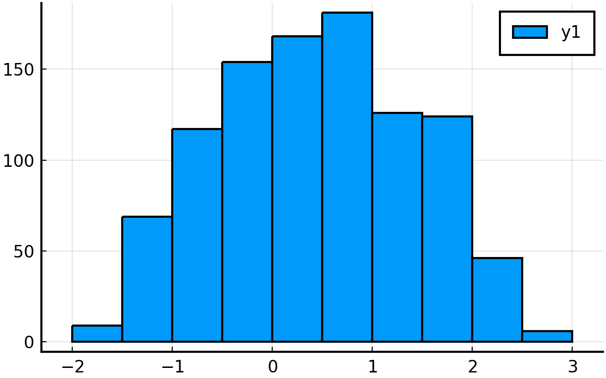
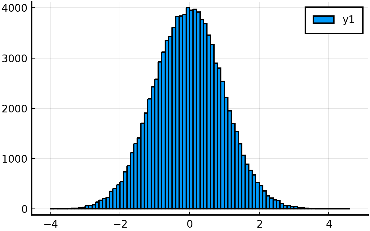
結果をヒストグラムで可視化
niter = 10^3
niter = 10^5
niter = 10^7
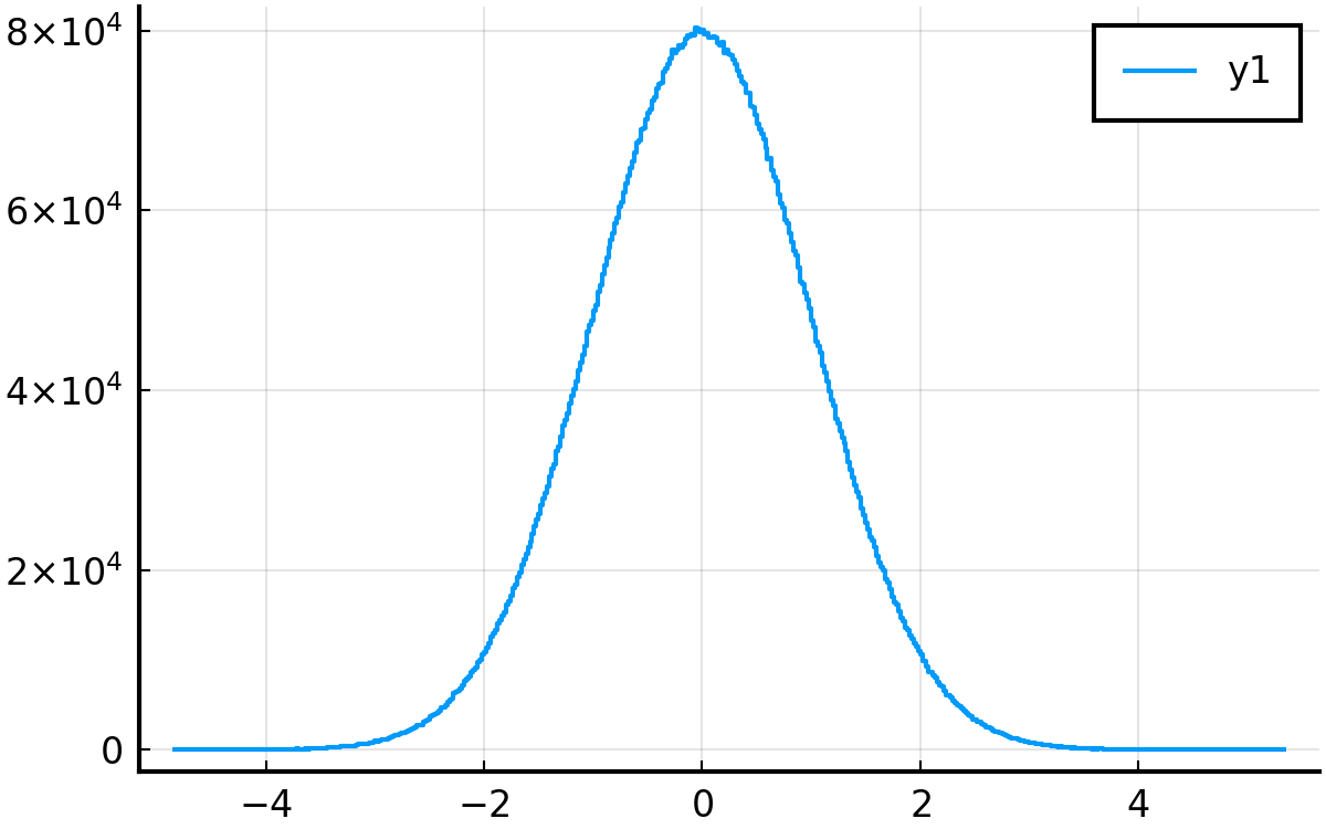
niter = 10^7では, 気を利かして普通のプロットのような図にしてくれたようです.
コード(click)
Julia
using Plots
xs = main(10^3);
pyplot(fmt=:svg, size=(400, 250))
histogram(xs)
PyPlot.savefig("ch4_1_1.png", dpi=300)
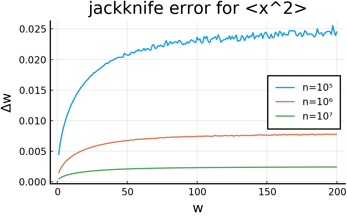
\( \langle x^2 \rangle \)のジャックナイフ誤差 ( p.60 )
p.60にあるジャックナイフ誤差を求める函数です. \( w \)の値の範囲変えられます.
Julia
function mcmcJackknife(xs, nw) # xs: sample, nw:wの最大値
  xs = xs.^2 # x^2の期待値なので
  f̄ = mean(xs) # total mean
  L = length(xs)
  Δw = zeros(1, nw)

  for w =  1:nw
    thisL = L - L%w
    n     = thisL / w
    thisXs = xs[1:thisL]
    thisXs = reshape(thisXs, w, :)
    l = mean(thisXs, dims=1)
    Δw[w] = sqrt(sum((l .- f̄).^2)/(n*(n-1)))

  end
  return Δw'
end
Metropolis法のサンプル数nの値を変えてプロットしてみました.
コード(click)
Julia
xs = main(10^5);
d1 = mcmcJackknife(xs, 200)

xs = main(10^6);
d2 = mcmcJackknife(xs, 200)

xs = main(10^7);
d3 = mcmcJackknife(xs, 200)

pyplot(fmt=:svg, size=(400, 250))
plot([d1 d2 d3], labels=["n=10⁵" "n=10⁶" "n=10⁷"])
xlabel!("w")
ylabel!("Δw")
title!("jackknife error for <x²>")
PyPlot.savefig("ch4_1_4jack.png", dpi=300)