『ゼロからできるMCMC』 Chapter 5をJuliaで

最終更新：2020/11/19

『ゼロからできるMCMC』 Chapter 5のコードを, 練習を兼ねてJuliaで書いてみました. 詳細なことを書くと著作権的にだめな気もするので, 解説などはありません.

Julia Version 1.5.0

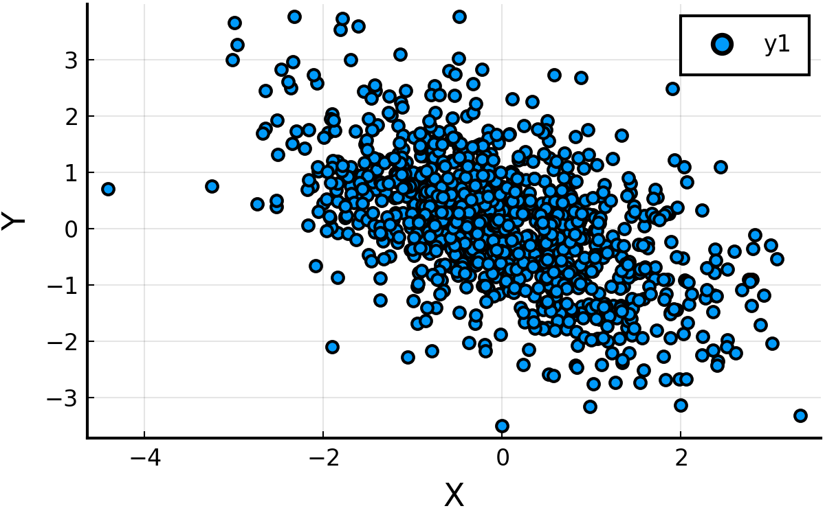
Metropolis法を用いた2次元正規分布からのサンプル ( p.80 )

Julia

using Random:seed!

function main(niter)

  seed!(12345)
  # step size
  step_size_x = 0.5
  step_size_y = 0.5

  # initial condition
  x = 0.0
  y = 0.0
  naccept = 0
  res = zeros(niter, 2)

  for iter in 1:niter

    backup_x = x
    backup_y = y
    action_init = 0.5*(x*x + y*y + x*y)

    x += (rand() - 0.5)*step_size_x*2.0
    y += (rand() - 0.5)*step_size_y*2.0
    action_fin =  0.5*(x*x + y*y + x*y)

    # Metropolis test
    metropolis = rand()
    if exp(action_init-action_fin) > metropolis
      naccept += 1
    else
      x = backup_x
      y = backup_y
    end
    res[iter, :] = [x y]
  end
  return res
end

resにサンプルを格納しました. 以下一部を選び出してプロット.

コード(click)

Julia

res = main(10^6);
pyplot(fmt=:svg, size=(400, 250))
scatter(res[1:1000:end, 1], res[1:1000:end, 2], xlabel = "X", ylabel = "Y")
PyPlot.savefig("ch5_1_1.png", dpi=300)

野球選手と物理学者の収入の期待値 ( p.83 )

それぞれの収入函数を定義して, 上の函数によるサンプルに適用してみた.

Julia

using Statistics
sphys(x) = (2 + tanh(x))/3 # 物理学者の収入函数
sbase(x) = x^2/2 * (x>2)   # 野球選手の収入函数

res = main(10^6)
meanPhys = mean(sphys.(res[:, 1]))
meanBase = mean(sbase.(res[:, 2]))

# 結果
julia> meanPhys
	0.664502877781731
julia> meanBase
	0.12487612365704041

この記事のTOP BACK TOP